|
|
| Linha 85: |
Linha 85: |
| | === Impedância de entrada, <math>Z_in</math> na linha sem perdas === | | === Impedância de entrada, <math>Z_in</math> na linha sem perdas === |
| | | | |
| − | Em relação a <math>Z_in</math> temos: | + | Em relação a <math>Z_{in}</math> temos: |
| | | | |
| | | | |
| − | ::::<math>Z_{in(z)}= Z_o { Z_L (e^{-\gamma z} + e^{\gamma z}) + Z_o(e^{-\gamma z} - e^{\gamma z}) \over Z_L (e^{-\gamma z} - e^{\gamma z}) + Z_o (e^{-\gamma z} + e^{\gamma z})}</math> | + | ::::<math>Z_{in(-l)}= Z_o { Z_L (e^{\gamma l} + e^{-\gamma l}) + Z_o(e^{\gamma l} - e^{-\gamma l}) \over Z_L (e^{\gamma l} - e^{-\gamma l}) + Z_o (e^{\gamma l} + e^{-\gamma l})}</math> |
| | | | |
| | | | |
| | | | |
| − | ::::<math>Z_{in(z)}= Z_o { Z_L ((e^{-\alpha z} e^{-j\beta z})+ (e^{\alpha z} e^{j\beta z})) + Z_o((e^{-\alpha z} e^{-j\beta z})- (e^{\alpha z} e^{j\beta z})) \over Z_L ((e^{-\alpha z} e^{-j\beta z}) - (e^{\alpha z} e^{j\beta z})) + Z_o ((e^{-\alpha z} e^{-j\beta z}) + (e^{\alpha z} e^{j\beta z}))}</math> | + | ::::<math>Z_{in}= Z_o { Z_L ((e^{\alpha l} e^{j\beta l})+ (e^{-\alpha l} e^{-j\beta l})) + Z_o((e^{\alpha l} e^{j\beta l})- (e^{-\alpha l} e^{-j\beta l})) \over Z_L ((e^{\alpha l} e^{j\beta l}) - (e^{-\alpha l} e^{-j\beta l})) + Z_o ((e^{\alpha l} e^{j\beta l}) + (e^{-\alpha l} e^{-j\beta l}))}</math> |
| | | | |
| | como α = 0: | | como α = 0: |
| | | | |
| | | | |
| − | ::::<math>Z_{in(z)}= Z_o { Z_L ( e^{-j\beta z}+ e^{j\beta z}) + Z_o( e^{-j\beta z}- e^{j\beta z}) \over Z_L ( e^{-j\beta z} - e^{j\beta z}) + Z_o ( e^{-j\beta z} + e^{j\beta z})}</math> | + | ::::<math>Z_{in}= Z_o { Z_L ( e^{j\beta l}+ e^{-j\beta l}) + Z_o( e^{j\beta l}- e^{-j\beta l}) \over Z_L ( e^{j\beta l} - e^{-j\beta l}) + Z_o ( e^{j\beta l} + e^{-j\beta l})}</math> |
| | | | |
| | | | |
| | e da identidade de Euler: | | e da identidade de Euler: |
| | | | |
| − | ::::<math>e^{-j\beta z} = cos \beta z - j sen \beta z</math> | + | ::::<math>e^{-j\beta l} = cos \beta l - j sen \beta l</math> |
| | | | |
| | | | |
| − | ::::<math>e^{j\beta z} = cos \beta z + j sen \beta z</math> | + | ::::<math>e^{j\beta z} = cos \beta l + j sen \beta l</math> |
| | | | |
| | | | |
| − | ::::<math>Z_{in(z)}= Z_o { Z_L ( cos \beta z {\color{red}- j sen \beta z} + cos \beta z {\color{red} + j sen \beta z)} + Z_o( {\color{red} cos \beta z} - j sen \beta z {\color{red}- cos \beta z} - j sen \beta z) \over Z_L ( {\color{red}cos \beta z} - j sen \beta z {\color{red} - cos \beta z} - j sen \beta z) + Z_o ( cos \beta z {\color{red} - j sen \beta z} + cos \beta z + {\color{red}j sen \beta z)}}</math> | + | ::::<math>Z_{in(z)}= Z_o { Z_L ( cos \beta l{\color{red}+ j sen \beta l} + cos \beta l {\color{red} - j sen \beta l)} + Z_o( {\color{red} cos \beta l} + j sen \beta l {\color{red}- cos \beta l} + j sen \beta l) \over Z_L ( {\color{red}cos \beta l} + j sen \beta l {\color{red} - cos \beta l} + j sen \beta l) + Z_o ( cos \beta l {\color{red} + j sen \beta l} + cos \beta l - {\color{red}j sen \beta l)}}</math> |
| | | | |
| | | | |
| | | | |
| − | ::::<math>Z_{in(z)}= Z_o { Z_L ( cos \beta z) - Z_o (jsen \beta z) \over -Z_L (jsen \beta z)+ Z_o (cos \beta z)}</math> | + | ::::<math>Z_{in}= Z_o { Z_L ( cos \beta l) + Z_o (jsen \beta l) \over Z_L (jsen \beta l)+ Z_o (cos \beta l)}</math> |
| | | | |
| − | dividindo numerador e denominador por cos βz: | + | dividindo numerador e denominador por <math>cos \beta l</math>: |
| | | | |
| | | | |
| | {| class="wikitable" style="margin: auto;color:black; background-color:#ffffcc;" cellpadding="10" | | {| class="wikitable" style="margin: auto;color:black; background-color:#ffffcc;" cellpadding="10" |
| − | |<math>Z_{in(z)}= Z_o { Z_L + jZ_o (tan \beta z) \over Z_o + jZ_L (tan \beta z)}</math> | + | |<math>Z_{in}= Z_o { Z_L + jZ_o (tan \beta l) \over Z_o + jZ_L (tan \beta l)}</math> |
| | |} | | |} |
Edição das 12h27min de 12 de setembro de 2015
Na linha de transmissão a propagação das ondas incidente e refletida cria um padrão de onda estacionária (figura 1).
figura 1: onda estacionária para uma linha sem perdas e com 
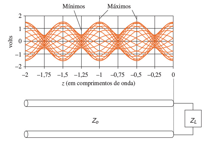
fonte: WENTWORTH, Stuart M. Eletromagnetismo Aplicado: Abordagem Antecipada das Linhas de Transmissão. Bookman, 2009.
O parâmetro utilizado para medir ou indicar a "quantidade" de onda estacionário ou de reflexão de onda numa linha de transmissão é a relação de onda estacionária (VSWR ou ROTE). O qual é definido como a razão entre as amplitudes máxima e a mínima da onda estacionária entre um pico e um vale consecutivo:


 (1)
(1)
substituindo  por
por  temos:


|
Linha sem perdas
Muitas linhas de transmissão são formadas por bons condutores e isolantes. Essas linhas apresentam valores de R e G muito pequenos e como:


Ao fazermos essas aproximações estamos considerando que a linha não tem perdas, como podemos observar no coeficiente de propagação (γ)


 (2)
(2)
como  e a equação (2) não apresenta parte real
  .
.
Impedância característica de uma linha sem perdas


 a impedância característica da uma linha sem perdas é resistiva !!! a impedância característica da uma linha sem perdas é resistiva !!!
|
Potência incidente de uma linha sem perdas
Uma vez que  é resistiva e , a potência incidente de uma linha sem perdas passa a ser:


|
Impedância de entrada,  na linha sem perdas
Em relação a  temos:


como α = 0:

e da identidade de Euler:


dividindo numerador e denominador por  :
:

|
