Mudanças entre as edições de "Transformação Bilinear"
| (7 revisões intermediárias por 2 usuários não estão sendo mostradas) | |||
| Linha 11: | Linha 11: | ||
Essa transformação é o resulta em um mapeamento exato do plano z no plano s através de <math> z = e^{sT} \ </math> | Essa transformação é o resulta em um mapeamento exato do plano z no plano s através de <math> z = e^{sT} \ </math> | ||
| + | {{collapse_top | Demonstração}} | ||
:<math> | :<math> | ||
\begin{align} | \begin{align} | ||
| Linha 16: | Linha 17: | ||
&= \frac{2}{T} \left[\frac{z-1}{z+1} + \frac{1}{3} \left( \frac{z-1}{z+1} \right)^3 + \frac{1}{5} \left( \frac{z-1}{z+1} \right)^5 + \frac{1}{7} \left( \frac{z-1}{z+1} \right)^7 + \cdots \right] \\ | &= \frac{2}{T} \left[\frac{z-1}{z+1} + \frac{1}{3} \left( \frac{z-1}{z+1} \right)^3 + \frac{1}{5} \left( \frac{z-1}{z+1} \right)^5 + \frac{1}{7} \left( \frac{z-1}{z+1} \right)^7 + \cdots \right] \\ | ||
&\approx \frac{2}{T} \frac{z - 1}{z + 1} \\ | &\approx \frac{2}{T} \frac{z - 1}{z + 1} \\ | ||
| − | & | + | &\approx \frac{2}{T} \frac{1 - z^{-1}}{1 + z^{-1}} |
\end{align} | \end{align} | ||
</math> | </math> | ||
| + | {{collapse_bottom}} | ||
| − | Ela pode ser utilizada para ser transformar um sistema linear invariante no tempo continuo <math> H_a(s) \ </math> em um sistema linear invariante no tempo discreto <math> H_d(z) \ </math>, e vice-versa. | + | Ela pode ser utilizada para ser transformar um sistema linear invariante no tempo continuo (filtro analógico) <math> H_a(s) \ </math> em um sistema linear invariante no tempo discreto (filtro digital) <math> H_d(z) \ </math>, e vice-versa. |
O mapeamento da função <math> H_a(s) \ </math> em <math> H_d(z) \ </math> é feita por: | O mapeamento da função <math> H_a(s) \ </math> em <math> H_d(z) \ </math> é feita por: | ||
| Linha 29: | Linha 31: | ||
\begin{align} | \begin{align} | ||
z &= e^{sT} \\ | z &= e^{sT} \\ | ||
| − | |||
&\approx \frac{1 + s T / 2}{1 - s T / 2} | &\approx \frac{1 + s T / 2}{1 - s T / 2} | ||
\end{align} | \end{align} | ||
</math> | </math> | ||
| − | ==A | + | {{collapse_top | Demonstração}} |
| + | :<math> | ||
| + | \begin{align} | ||
| + | &z = e^{sT} \\ | ||
| + | \text{foi visto que} \\ | ||
| + | &s \approx \frac{2}{T} \frac{z - 1}{z + 1} \\ | ||
| + | \text{então rearranjando z} \\ | ||
| + | &s T / 2(z + 1) \approx (z - 1) \\ | ||
| + | &(s T / 2) z + s T / 2 \approx z - 1 \\ | ||
| + | |||
| + | &1 + s T / 2 \approx z(1 - s T / 2) \\ | ||
| + | \text{portanto} \\ | ||
| + | &z \approx \frac{1 + s T / 2}{1 - s T / 2} | ||
| + | \end{align} | ||
| + | </math> | ||
| + | |||
| + | {{collapse_bottom}} | ||
| + | |||
| + | == Empenamento de frequência (''frequency warping'') == | ||
| + | |||
| + | Determinar a resposta de frequência em filtro analógico (de tempo contínuo), a função de transferência <math> H_a(s) </math> é avaliada em <math>s = j \omega_a </math>, que corresponde aos valores dessa função no eixo imaginário <math> j \omega </math>. Da mesma forma para filtros digitais (de tempo discreto), a função de transferência <math> H_d(z) </math> é avaliada em <math>z = e^{ j \omega_d T} </math>, correspondendo aos valores sobre o circulo unitário pois <math>z = e^{ j \omega_d T} </math> possui magnitude constante <math> |z| = 1 </math>. | ||
| + | |||
| + | A transformação bilinear mapeia o eixo imaginário do plano ''s'' no circulo unitário no plano ''z'', no entanto o mapeamento das frequências não é linear, sofrendo um empenamento (distorção). Para utilizar essa transformação na obtenção de filtros digitais a partir de filtros analógicos, é necessário determinar como cada frequencia do filtro final desejado <math> \omega_d </math> deve ser projetada no filtro analógico <math> \omega_a </math>. Essa distorção pode ser obtida fazendo a substituição de <math>z = e^{ j \omega_d T} \ </math> na equação da transformação bilinear, e aplicando a [https://en.wikipedia.org/wiki/Euler's_formula#Relationship_to_trigonometry fórmula de Euler para o seno]. | ||
| + | :<math>H_d(z) = H_a \left( \frac{2}{T} \frac{z-1}{z+1}\right) </math> | ||
| + | |||
| + | : <math>H_d(e^{ j \omega_d T}) = H_a \left(j \frac{2}{T} \cdot \tan \left( \omega_d T/2 \right) \right) = H_a(j \omega_a) </math> | ||
| + | |||
| + | {{collapse_top | Demonstração}} | ||
| + | Considere que: | ||
| + | :<math>\begin{align} | ||
| + | 2 \cos \omega = e^{j\omega} + e^{-j\omega}, \\ | ||
| + | 2j \sin \omega = e^{j\omega} - e^{-j\omega}. | ||
| + | \end{align}</math> | ||
| + | |||
| + | e que | ||
| + | :<math>\tan \omega =\frac{\sin \omega}{\cos \omega} </math>, e | ||
| + | |||
| + | :<math> 1 = e^{\omega}e^{-\omega} \ </math> | ||
| + | |||
| + | |||
| + | É possível mostrar que: | ||
| + | |||
| + | {| | ||
| + | |- | ||
| + | |<math>H_d(e^{ j \omega_d T}) </math> | ||
| + | |<math>= H_a \left( \frac{2}{T} \frac{e^{ j \omega_d T} - 1}{e^{ j \omega_d T} + 1}\right) </math> | ||
| + | |- | ||
| + | |<math>H_d(e^{ j \omega_d T}) </math> | ||
| + | |<math>= H_a \left( \frac{2}{T} \frac{e^{j \omega_d T/2}e^{j \omega_d T/2} - e^{j \omega_d T/2}e^{-j \omega_d T/2}}{e^{j \omega_d T/2}e^{j \omega_d T/2} + e^{j \omega_d T/2}e^{-j \omega_d T/2}}\right) </math> | ||
| + | |- | ||
| + | | | ||
| + | |<math>= H_a \left( \frac{2}{T} \cdot \frac{e^{j \omega_d T/2} \left(e^{j \omega_d T/2} - e^{-j \omega_d T/2}\right)}{e^{j \omega_d T/2} \left(e^{j \omega_d T/2} + e^{-j \omega_d T/2 }\right)}\right) </math> | ||
| + | |- | ||
| + | | | ||
| + | |<math>= H_a \left( \frac{2}{T} \cdot \frac{\left(e^{j \omega_d T/2} - e^{-j \omega_d T/2}\right)}{\left(e^{j \omega_d T/2} + e^{-j \omega_d T/2 }\right)}\right) </math> | ||
| + | |- | ||
| + | | | ||
| + | |<math>= H_a \left(\frac{2}{T} \cdot \frac{2j \sin(\omega_d T/2) }{2 \cos(\omega_d T/2) }\right) </math> | ||
| + | |- | ||
| + | | | ||
| + | |<math>= H_a \left(j \frac{2}{T} \cdot \tan \left( \omega_d T/2 \right) \right) </math> | ||
| + | |- | ||
| + | | | ||
| + | |<math>= H_a(j \omega_a) </math>, onde <math> \omega_a = \frac{2}{T} \tan \left( \omega_d \frac{T}{2} \right) </math> | ||
| + | |} | ||
| + | |||
| + | {{collapse bottom}} | ||
| + | |||
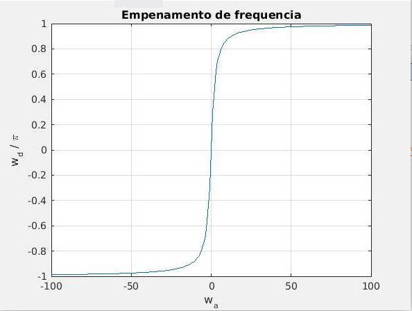
| + | Isso mostra que cada ponto no circulo unitário do plano ''z'' é mapeado em um ponto no eixo imaginário do plano ''s''. E que as frequências do filtro digital são mapeadas nas frequencias analógicas pela equação: | ||
| + | |||
| + | :<math> \omega_a = \frac{2}{T} \tan \left( \omega_d \frac{T}{2} \right) </math> | ||
| + | |||
| + | <!-- | ||
| + | Apesar desse empenamento, os ganhos e mudanças de fase do filtro digital em <math> (2/T) \tan(\omega_d T/2) </math> são exatamente as mesmas do filtro analógico, | ||
| + | |||
| + | |||
| + | The discrete-time filter behaves at frequency <math>\omega_d</math> the same way that the continuous-time filter behaves at frequency <math> (2/T) \tan(\omega_d T/2) </math>. Specifically, the gain and phase shift that the discrete-time filter has at frequency <math>\omega_d</math> is the same gain and phase shift that the continuous-time filter has at frequency <math>(2/T) \tan(\omega_d T/2)</math>. This means that every feature, every "bump" that is visible in the frequency response of the continuous-time filter is also visible in the discrete-time filter, but at a different frequency. For low frequencies (that is, when <math>\omega_d \ll 2/T</math> or <math>\omega_a \ll 2/T</math>), then the features are mapped to a ''slightly'' different frequency; <math>\omega_d \approx \omega_a </math>. | ||
| + | |||
| + | One can see that the entire continuous frequency range | ||
| + | --> | ||
| + | Além disso a faixa infinita de frequências do filtro analógico | ||
| + | : <math> -\infty < \omega_a < +\infty \ </math> | ||
| − | + | é mapeada no filtro digital no intervalo limitado | |
| + | : <math> -\frac{\pi}{T} < \omega_d < +\frac{\pi}{T}. </math> | ||
| + | <center> | ||
| + | :'''Figura - Empenamento de frequencia resultado da transformada Bilinear, para T = 1''' | ||
| + | :[[Arquivo:EmpenamtoFreqBilinear1.png | 400px]] [[Arquivo:EmpenamtoFreqBilinear2.png | 400px]] </center> | ||
| + | <!-- | ||
| − | == | + | The continuous-time filter frequency <math> \omega_a = 0 </math> corresponds to the discrete-time filter frequency <math> \omega_d = 0 </math> and the continuous-time filter frequency <math> \omega_a = \pm \infty </math> correspond to the discrete-time filter frequency <math> \omega_d = \pm \pi / T. </math> |
| + | One can also see that there is a nonlinear relationship between <math> \omega_a \ </math> and <math> \omega_d.</math> This effect of the bilinear transform is called '''frequency warping'''. The continuous-time filter can be designed to compensate for this frequency warping by setting <math> \omega_a = \frac{2}{T} \tan \left( \omega_d \frac{T}{2} \right) </math> for every frequency specification that the designer has control over (such as corner frequency or center frequency). This is called '''pre-warping''' the filter design. | ||
| − | + | It is possible, however, to compensate for the frequency warping by pre-warping a frequency specification <math> \omega_0 </math> (usually a resonant frequency or the frequency of the most significant feature of the frequency response) of the continuous-time system. These pre-warped specifications may then be used in the bilinear transform to obtain the desired discrete-time system. When designing a digital filter as an approximation of a continuous time filter, the frequency response (both amplitude and phase) of the digital filter can be made to match the frequency response of the continuous filter at a specified frequency <math> \omega_0 </math>, as well as matching at DC, if the following transform is substituted into the continuous filter transfer function.<ref>{{cite book |last=Astrom |first=Karl J. |date=1990 |title=Computer Controlled Systems, Theory and Design |edition=Second |publisher=Prentice-Hall |page=212 |isbn=0-13-168600-3}}</ref> This is a modified version of Tustin's transform shown above. | |
| − | <math> | + | :<math>s \leftarrow \frac{\omega_0}{\tan\left(\frac{\omega_0 T}{2}\right)} \frac{z - 1}{z + 1}.</math> |
| − | + | However, note that this transform becomes the original transform | |
| + | :<math>s \leftarrow \frac{2}{T} \frac{z - 1}{z + 1}</math> | ||
| − | + | as <math> \omega_0 \to 0 </math>. | |
| − | |||
| + | The main advantage of the warping phenomenon is the absence of aliasing distortion of the frequency response characteristic, such as observed with [[Impulse invariance]]. | ||
| − | + | --> | |
| − | + | ==FONTES== | |
| + | *[https://www.mathworks.com/help/control/ug/continuous-discrete-conversion-methods.html#bs78nig-8 Continuous-Discrete Conversion Methods Tustin Approximation] Mathworks | ||
Edição atual tal como às 13h30min de 23 de abril de 2020
Discretização de filtros analógicos
A transformação bilinear do domínio da Transformada de Laplace para o domínio da Transformada z é feito por

O mapeamento inverso em é feita por


é uma aproximação de primeira ordem do logaritmo pela série de potência

Essa transformação é o resulta em um mapeamento exato do plano z no plano s através de

| Demonstração |
|---|
|
|
![{\displaystyle {\begin{aligned}s&={\frac {1}{T}}\ln(z)\\&={\frac {2}{T}}\left[{\frac {z-1}{z+1}}+{\frac {1}{3}}\left({\frac {z-1}{z+1}}\right)^{3}+{\frac {1}{5}}\left({\frac {z-1}{z+1}}\right)^{5}+{\frac {1}{7}}\left({\frac {z-1}{z+1}}\right)^{7}+\cdots \right]\\&\approx {\frac {2}{T}}{\frac {z-1}{z+1}}\\&\approx {\frac {2}{T}}{\frac {1-z^{-1}}{1+z^{-1}}}\end{aligned}}}](https://en.wikipedia.org/api/rest_v1/media/math/render/svg/5fb3a0ef3b4b9ba5baa49d864f7242a1a39761f5)
Ela pode ser utilizada para ser transformar um sistema linear invariante no tempo continuo (filtro analógico) em um sistema linear invariante no tempo discreto (filtro digital) , e vice-versa. O mapeamento da função em é feita por:

O mapeamento inverso em é feita pela aproximação de primeira ordem da substituição

| Demonstração |
|---|
|
|

Empenamento de frequência (frequency warping)
Determinar a resposta de frequência em filtro analógico (de tempo contínuo), a função de transferência é avaliada em , que corresponde aos valores dessa função no eixo imaginário . Da mesma forma para filtros digitais (de tempo discreto), a função de transferência é avaliada em , correspondendo aos valores sobre o circulo unitário pois possui magnitude constante .


A transformação bilinear mapeia o eixo imaginário do plano s no circulo unitário no plano z, no entanto o mapeamento das frequências não é linear, sofrendo um empenamento (distorção). Para utilizar essa transformação na obtenção de filtros digitais a partir de filtros analógicos, é necessário determinar como cada frequencia do filtro final desejado deve ser projetada no filtro analógico . Essa distorção pode ser obtida fazendo a substituição de na equação da transformação bilinear, e aplicando a fórmula de Euler para o seno.


| Demonstração | ||||||||||||||
|---|---|---|---|---|---|---|---|---|---|---|---|---|---|---|
|
Considere que: e que
|


Isso mostra que cada ponto no circulo unitário do plano z é mapeado em um ponto no eixo imaginário do plano s. E que as frequências do filtro digital são mapeadas nas frequencias analógicas pela equação:
Além disso a faixa infinita de frequências do filtro analógico

é mapeada no filtro digital no intervalo limitado

- Figura - Empenamento de frequencia resultado da transformada Bilinear, para T = 1